Training Set Audit

Training Set Audit inspects the active training data in two stages: it first finds technical problems that can block training, then shows how composition, labels, local environments, structural phases, and magnetic types are distributed within the dataset. Every result keeps the original structure indices so that you can return to NEP Dataset Display to inspect, select, or export the affected structures.

This page reports evidence from the current dataset snapshot. A training set alone cannot prove complete coverage of physical space, and model reliability cannot be established without independent test data.

Open the audit from NEP Dataset Display

Load the training data in NEP Dataset Display, then use either entry point:

Entry point	Opens	Use it for
Title-bar Save split menu → Check current dataset	Training Set Audit → Overview	Run the complete audit on the active structures
Plot toolbar → Explore distributions	Data map → Data distribution	Inspect distributions of energy, force, virial, predictions, or errors

If no data is loaded, NepTrainKit asks you to open a dataset first. The audit covers the active structures only; structures already removed from the dataset are outside the audit scope.

Re-run the audit after the data changes

The header records the audited structure range, data fingerprint, and generation time. Click Re-run checks after deleting structures, switching datasets, editing labels, or changing nep.txt. An earlier result no longer represents the modified data.

Recommended workflow

Step 1: Start with Overview

The Overview answers three questions:

• Are there empty structures, non-finite values, invalid label shapes, or other training blockers?

• Which exact compositions, elements, and labels are present?

• Which high-force, high-energy, repeated, or low-frequency groups deserve review first?

Select a review topic to see the observation, interpretation, and capability boundary. Use the structure button to return to NEP Dataset Display with the affected structures selected.

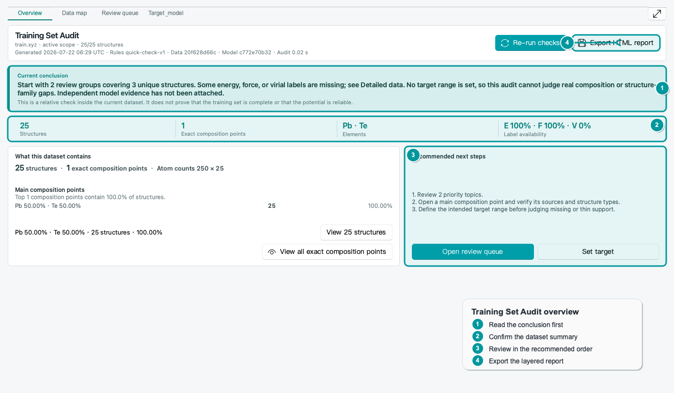
Follow the numbered reading order in the screenshot: read the current conclusion, confirm how many structures and labels were checked, then use Recommended next steps to enter the review queue. Export HTML only when you need a durable record or a report for a collaborator.

Step 2: Inspect composition, structural phase, and magnetic type in Data map

The composition map groups structures by exact atomic ratio. For example, Fe2Ni2, Fe4Ni4, and Fe32Ni32 all belong to the same Fe:Ni = 1:1 composition point. The table still records the number of structures, atom counts, and Config_type, so structures with different cell sizes are not treated as the same geometry.

On first entry, bar height represents the number of structures at that concentration. After the basic diagnostics appear, the page automatically scans all structures in the current audit scope in the background; no separate start button is required. For large systems, disable Automatically analyze structure evidence under Settings > Personalization if automatic analysis is not desired. Two additional views become available when analysis finishes, without changing the current composition view automatically:

• Structural phase: FCC, HCP, and BCC, plus conservatively confirmed A4, L1₀, L1₂, B1, B2, B3, B4, C1, B8₁, D0₃, L2₁, C1ᵦ, D0₁₉, C14, and C15 prototypes; all remaining structures are shown as mixed local structure or unresolved;

• Magnetic type: FM, AFM (unsubtyped), layered AFM (↑↓), double-layer AFM (↑↑↓↓), FiM, PM-like (spin-disordered), other noncollinear, unresolved, low/zero moment, and no valid spin field.

When analysis finishes, select a composition and refine it with the structural-phase and magnetic-type filters. Click Show selected structures to return to NEP Dataset Display.

Structural phase and magnetism are independent evidence layers. The same FCC or BCC framework can carry different magnetic structures, so the interface does not collapse them into a single inseparable label. Config_type is source metadata only and does not participate in structural-phase or magnetic-type classification.

Under Advanced evidence → Magnetic order, switch among three 100% stacked charts normalized by structure-frame count: magnetic-type shares within each structural phase, structural-phase shares within each magnetic type, and magnetic-type shares across the full audit scope. Percentages inside colored segments show the share, counts at the right show the number of frames, and clicking a segment selects its structures.

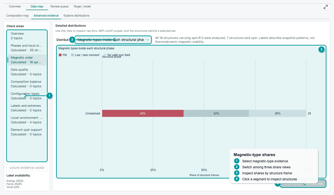
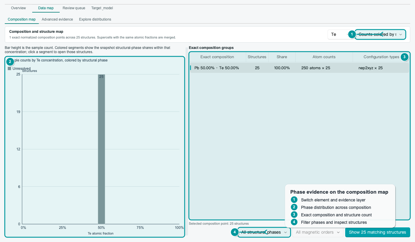
The example above contains a single exact Pb:Te = 1:1 composition point. Neither a-CNA nor a built-in prototype template provides strong evidence, so the bar is gray and labeled unresolved. This is not an analysis failure: the current geometric evidence is insufficient for a supported label. With valid spin:R:3 data, a magnetic-order coloring option appears in the evidence selector and the magnetic filter becomes available.

Step 3: Trace local environments in Advanced evidence

With an active nep.txt, the audit reads the model elements and radial/angular cutoffs, then measures the neighborhoods that the model can actually see:

• coordination numbers and neighboring-element composition around each central element;

• whether element pairs merely coexist or actually come into contact inside the cutoff;

• label distributions, the high-force tail, and the high-energy tail.

Without nep.txt, data quality, composition, labels, structural phase, and magnetic type remain available. Local-chemistry and element-pair contact checks that require model cutoffs are marked unavailable.

Step 4: Record decisions in Review queue

The Review queue combines related low-frequency bins into one topic instead of producing many alerts for the same issue. Available states depend on the finding: blockers can be marked unresolved or resolved and rechecked; repeated geometries can be intentionally retained, isolated as candidates, or sent for recalculation; ordinary review groups can be marked physically expected or scheduled for geometry inspection. These states document the review of the current snapshot. They do not delete or modify structures.

Step 5: Use Target & model only after defining the research scope

A target comparison is meaningful only after the user declares a target. You can specify:

• a concentration range for one element;

• required concentration points;

• required Config_type values;

• a minimum structure count at each point.

The comparison evaluates exact composition points and structure-count rules. A point marked supported has passed those count rules only; it does not prove coverage of local environments, temperature-pressure paths, defect types, or model accuracy.

Show NEP predictions on the current training data are useful for browsing errors, but they are not automatically treated as independent model validation. Generalization error requires separately mapped reference and prediction values with verified units.

What the quick audit checks

Training blockers

The following results violate explicit data contracts and should be resolved before training:

• empty structures;

• NaN / Inf in positions, cells, or labels;

• invalid array shapes for positions, forces, virial, or related fields;

• periodic directions that are inconsistent with the cell;

• unknown elements, or an element count that does not match the atom count;

• a conservative overlap signal when the shortest interatomic distance is below 0.5 Å;

• identical geometries with mutually inconsistent energy, force, or virial labels.

Geometry identity includes elements, periodic boundaries, cell, and coordinates; cells and coordinates are rounded to eight decimal places for comparison. Current absolute tolerances for conflicting labels are 1 × 10⁻⁵ for energy, 1 × 10⁻⁵ for force, and 1 × 10⁻⁴ for virial, with zero relative tolerance.

NepTrainKit does not delete blocking structures or decide which repeated calculation is correct. Check the structure provenance and original DFT output first.

Recommended review groups

• the highest 10% by maximum force;

• the highest 5% by energy per atom;

• repeated geometries;

• low-frequency compositions, local environments, or imbalanced groups inside the current dataset.

Rank-based percentile groups exist by construction. High-force, high-energy, or repeated structures may represent intended physics, explicit weighting, or independent calculations. Treat these findings as review entry points, not deletion recommendations.

How structural phases are identified

FCC, HCP, and BCC: adaptive common-neighbor analysis

The audit applies adaptive common-neighbor analysis (a-CNA) to each atom. A periodic neighbor search collects up to 24 neighbors, then determines an atom-specific cutoff from the gap between the first and second neighbor shells.

For FCC and HCP, let the sorted neighbor distances be \(d_1 \le \cdots \le d_{13}\). Only when

\[ \frac{d_{13}}{d_{12}} \ge 1.08 \]

does the analysis use

\[ r_\mathrm{cut}=\frac{d_{12}+d_{13}}{2} \]

to separate the 12-fold first-neighbor shell. Each center-neighbor bond is then described by three CNA values: the number of common neighbors, the number of bonds among those common neighbors, and the longest bond-chain length. The ideal topologies are:

Local structure	CNA signature
FCC	12 bonds of (4, 2, 1)
HCP	6 bonds of (4, 2, 1) + 6 bonds of (4, 2, 2)
BCC	6 bonds of (4, 4, 3) + 8 bonds of (6, 6, 5)

BCC uses the first 14 neighbors and requires \(d_{15}/d_{14} \ge 1.08\). Atoms that fail the shell-gap or topology tests are labeled unresolved rather than forced into the nearest crystal class.

For a structure, the fraction of atoms assigned to local phase \(\alpha\) is

\[ p_\alpha=\frac{N_\alpha}{N} \]

Unless a more specific ordered phase has been confirmed, \(p_\alpha \ge 0.80\) is strong structural evidence, \(0.50 \le p_\alpha < 0.80\) is mixed evidence, and a value below 0.50 is unresolved. These fractions describe local topology in the saved snapshot; they are not thermodynamic phase fractions.

Common crystal prototypes: geometry and chemistry must both pass

Ordered alloys and compounds cannot be distinguished from FCC/HCP/BCC local geometry alone. For three-dimensionally periodic structures, the audit conservatively checks composition, local shape, and species occupancy together. The catalog below contains common prototypes tested against competing structures; it is not a complete crystallographic database.

Display label	Common name	Pearson / space group	Description
A4	Diamond	cF8 / \(Fd\bar 3m\) (227)	Single-element tetrahedral network
L1₀	CuAu type	tP2 / \(P4/mmm\) (123)	FCC-derived 1:1 ordered structure
L1₂	Cu₃Au type	cP4 / \(Pm\bar 3m\) (221)	FCC-derived 3:1 ordered structure
B1	Rock salt	cF8 / \(Fm\bar 3m\) (225)	1:1 octahedral coordination
B2	CsCl	cP2 / \(Pm\bar 3m\) (221)	BCC-derived 1:1 ordered structure
B3 / B4	Zinc blende / wurtzite	cF8 / \(F\bar 43m\) (216)；hP4 / \(P6_3mc\) (186)	Cubic / hexagonal tetrahedral compounds
C1	Fluorite	cF12 / \(Fm\bar 3m\) (225)	1:2 compound
B8₁	NiAs	hP4 / \(P6_3/mmc\) (194)	Hexagonal 1:1 compound
D0₃	Fe₃Al type	cF16 / \(Fm\bar 3m\) (225)	BCC-derived 3:1 ordered structure
L2₁ / C1ᵦ	Full-Heusler / half-Heusler	cF16 / \(Fm\bar 3m\) (225)；cF12 / \(F\bar 43m\) (216)	Ternary 2:1:1 / 1:1:1 structures
D0₁₉	Ni₃Sn type	hP8 / \(P6_3/mmc\) (194)	HCP-derived 3:1 ordered structure
C14 / C15	Laves	hP12 / \(P6_3/mmc\) (194)；cF24 / \(Fd\bar 3m\) (227)	1:2 Frank-Kasper structure

The local-shape comparison first removes the overall length scale. For the selected \(K\) neighbors, distances are normalized by their mean \(\bar r\) to construct

\[ \mathbf d=\operatorname{sort}\left(\frac{r_i}{\bar r}\right) \oplus \operatorname{sort}\left(\frac{\lVert\mathbf r_i-\mathbf r_j\rVert}{\bar r}\right)_{i<j} \]

Here \(\oplus\) concatenates the two sorted sets. The audit computes the minimum root-mean-square distance between this descriptor and built-in reference-crystal templates. Species checks use the same complete neighbor shells and compare element-role counts in every shell. This tolerates translation, rotation, uniform scaling, atom reordering, species-ID relabeling, and moderate distortion, but does not assign a prototype from stoichiometry, lattice constants, or a merely cubic-looking cell.

For the common-prototype gate, composition may differ from the ideal ratio by at most 3.5%; at least 0.82 of atoms must pass geometry, 0.80 must pass chemistry, and 0.80 must pass both. Each local environment uses at least 14 neighbors without truncating a complete shell. Near a shell boundary, at most max(1, floor(0.08 K)) neighbor-ordering exchanges are tolerated. If two passing candidates are not clearly separated by local-shape distance or joint support, the result is unresolved rather than a nearest-template guess.

• L1₂: identify a binary composition close to A:B = 1:3. In addition to an FCC-like shape, an A site must have no A atoms among its first 12 neighbors and six A atoms in the second shell; a B site must have four A atoms in the first 12 neighbors and no A atoms in the second shell. At least 0.80 of sites must pass geometry, 0.85 must pass chemistry, and 0.80 must pass both.

• Laves: identify a binary composition close to A:B = 1:2. A sites are checked against a Z16 template and B sites against a Z12 template. An A site should have four A neighbors and a B site should have six A neighbors. Both the geometry pass fraction and the joint geometry-and-chemistry fraction must be at least 0.85. C14 and C15 are then separated using the centrosymmetry parameter of the B sublattice.

C15 has Pearson symbol cF24 and space group \(Fd\bar 3m\). The F denotes a face-centered cubic Bravais lattice; it does not make the structure an A1 FCC solid solution or give every atom an FCC a-CNA neighborhood. The two C15 sites instead use the Z12/Z16 Frank–Kasper environments of a Laves phase. The interface can therefore report both C15 Laves confirmed and a-CNA (FCC/HCP/BCC only): other / unresolved. See the AFLOW C15 prototype.

When A/B roles are inferred automatically, the actual minority-element fraction must be within 3.5% of the ideal composition. C36 local stacking can be indistinguishable from mixed C14/C15 under the current local evidence, so it is reported only as an unconfirmed signal rather than a confirmed C36 label. Unconfirmed means insufficient evidence, not proof that the phase is absent.

Why B1 confirmed and local unresolved can appear together

The two lines answer different questions. For a slightly strained and displaced U₄N₄ structure, the species-resolved complete neighbor shells still match the B1 rock-salt template, so the structure-level label can show:

::

a-CNA recognizes only per-atom A1-FCC, A2-BCC, or A3-HCP local topology. Every atom in B1 has a six-fold octahedral first shell rather than a 12-fold A1-FCC environment, so the same card can also show:

::

These statements do not conflict, and B1 has not been mislabeled as FCC. The first is compound-prototype confirmation; the second is a per-atom local metallic-framework statistic. NepTrainKit preserves both evidence layers. Specific prototypes not yet in the confirmation catalog, such as A15, perovskite, L1₁, and C36, are not guessed as a supported prototype. If they still have a clear FCC/BCC/HCP local framework, the page reports only that framework.

How magnetic types are identified

Input requirement

Magnetic-type analysis reads only per-atom spin:R:3: one three-component spin vector for each atom.

Properties=species:S:1:pos:R:3:spin:R:3

spin must be a numeric N × 3 array with finite components. mforce and force_mag are magnetic-force labels and cannot replace spin. A structure without valid spin data is reported as having no valid spin field; it is not guessed to be nonmagnetic.

Four groups of observables

Let the spin on atom \(i\) be \(\mathbf s_i\), its magnitude be \(m_i=\lVert\mathbf s_i\rVert\), and its unit direction be \(\hat{\mathbf s}_i=\mathbf s_i/m_i\). Moments at or below 1 × 10⁻⁷ are excluded from directional statistics.

1. Net-moment ratio

   \[ R_M=\frac{\left\lVert\sum_i\mathbf s_i\right\rVert}{\sum_i\lVert\mathbf s_i\rVert} \]

   \(R_M\) near 1 indicates net alignment, while a value near 0 indicates global compensation. The ratio is dimensionless; the mean moment retains the unit of the input spin vectors.

2. Collinearity and coplanarity

   \[ \mathbf Q=\frac{1}{N_s}\sum_i\hat{\mathbf s}_i\hat{\mathbf s}_i^{\mathsf T}, \qquad \lambda_1\le\lambda_2\le\lambda_3 \]

   Collinearity is \(C=\lambda_3\) and coplanarity is \(P=1-3\lambda_1\). A value of \(C\) near 1 means the directions concentrate around one axis; \(P\) near 1 means the directions lie mainly in one plane.

3. Neighbor spin correlation

   For each atom, the audit takes up to 12 nearest neighbors and computes

   \[ \bar c=\left\langle\hat{\mathbf s}_i\cdot\hat{\mathbf s}_j\right\rangle_{\langle i,j\rangle} \]

   A dot product of at least 0.80 counts as a parallel neighbor, while a value at or below -0.80 counts as antiparallel. The parallel and antiparallel neighbor fractions are also recorded.

4. Low-order magnetic structure factor

   For fractional coordinates \(\mathbf f_i\), the audit scans nonzero integer wave vectors with \(|h|,|k|,|l|\le3\) along periodic directions and computes

   \[ S(\mathbf q)=\min\!\left[1, \frac{2\left\lVert\sum_i\mathbf s_i \exp\!\left(\mathrm i2\pi\mathbf q\cdot\mathbf f_i\right)\right\rVert^2} {\left(\sum_i m_i\right)^2}\right] \]

   The page records the maximum \(S_\mathrm{max}\) and its integer wave vector. This detects low-order modulation that the current supercell can represent; it is not a continuous reciprocal-space scan.

Structure-level magnetic-type labels

The first matching rule in the following table is used:

Output label	Current criterion
Low / zero moment	No valid moment is greater than 1 × 10⁻⁷
Unresolved	Only one valid moment, or insufficient evidence for any other type
FM	\(C\ge0.90\), \(R_M\ge0.82\), and \(\bar c\ge0.20\)
AFM	\(C\ge0.90\), \(R_M\le0.20\), and at least one of: \(S_\mathrm{max}\ge0.45\), \(\bar c\le-0.25\), or an antiparallel-neighbor fraction of at least 0.20
FiM	\(C\ge0.90\), \(R_M<0.82\), an antiparallel-neighbor fraction of at least 0.20, and either \(S_\mathrm{max}\ge0.35\) or \(\bar c<-0.05\)
Other noncollinear	\(C<0.90\) and either both \(S_\mathrm{max}\ge0.45\) and \(P\ge0.72\), or at least one of \(S_\mathrm{max}\ge0.32\) and \(\lvert\bar c\rvert\ge0.30\)
PM-like (spin-disordered)	\(R_M\le0.25\), \(S_\mathrm{max}\le0.22\), and \(\lvert\bar c\rvert\le0.15\)

The program checks layer sequences only after the structure-level result is AFM. It groups atoms whose fractional-coordinate separation along the same periodic direction is at most 0.025 into one magnetic layer and requires an absolute within-layer polarization of at least 0.80. Subtype recognition requires at least four atoms with valid moments. One complete ↑↓ period is labeled layered AFM, while ↑↑↓↓ is labeled double-layer AFM. Periodic boundaries repeat the sequence, so a second copy inside the same cell is unnecessary. AFM structures that do not pass the layer-sequence gate are shown as AFM (unsubtyped).

Per-element results use the same net moment, direction tensor, same-element neighbor correlation, and structure factor to label each snapshot as aligned, compensated, modulated, noncollinear, mixed collinear, or disordered. Neighboring unlike-element coupling is classified from the mean dot product: at least 0.50 is parallel, at most -0.50 is antiparallel, and intermediate values are mixed.

Limits of magnetic-type labels

These labels describe a single saved spin snapshot, not a finite-temperature magnetic phase. PM-like means only that this frame has low net moment, a weak q peak, and weak neighbor correlation under the current criteria; it does not establish a thermodynamic paramagnetic phase. The wave-vector scan covers only low-order integer points representable in the current supercell. Incommensurate spirals, longer-period modulation, strongly defective structures, or very small cells may be reported as other noncollinear or unresolved. Transition temperatures, domain stability, and free energies require separate simulations and physical validation.

Export an HTML report

Click Export HTML report in the page header to save the current audit snapshot. The report follows the same reading priority as the application instead of expanding every raw table at once:

1. The first screen states whether action is required before training, review is recommended, or no blocker was found.

2. Summary cards show the structure count, exact-composition count, blocker count, review-group count, and phase/magnetic analysis progress.

3. Start here lists at most the three highest-priority findings and gives the next action for each.

4. Complete findings are grouped into Required action, Review next, Supporting evidence, and Unavailable checks. Only blocking findings are expanded by default.

5. Ordinary review details, composition inventory, phase/magnetic maps, input parameters, and run fingerprints remain collapsed until evidence is needed.

Read the status banner and Start here first, then expand only the evidence needed for the decision. The report still preserves:

• audit scope, generation time, and data/model fingerprints;

• summaries of data quality, composition, labels, local environments, structural phase, and magnetic type;

• the original structure indices associated with each finding;

• the rule and capability boundary for every finding.

The report is a record for review and collaboration. It is not proof of global coverage and does not issue automatic sampling instructions.

Questions this audit cannot answer by itself

Training Set Audit cannot determine by itself:

• whether the data cover a target temperature, pressure, defect, interface, or phase-transition regime;

• which target structure is definitely missing;

• the potential error on an independent test set;

• whether long molecular-dynamics trajectories will remain stable;

• whether an error in a particular property is acceptable;

• whether the thermodynamic structural or magnetic phase represented by a single snapshot is stable.

Those questions require a declared target space, target structures or trajectories, model predictions, independent reference data, and a property-specific validation protocol. Rare in this dataset means relatively infrequent inside the current snapshot; it does not mean missing from the research target.